Introduction
A backtest produces a point estimate—an annualized Sharpe ratio, a maximum drawdown—and a point estimate invites a confidence interval. The advice circulating in practitioner writing is appealingly simple: resample the backtest’s daily returns, or its individual trades, with replacement; recompute the statistic on each resample; and read the interval off the quantiles of the bootstrap distribution [1].1 The procedure inherits the prestige of the bootstrap [4] while quietly discarding its central assumption: resampling individual observations is justified for independent data, and strategy PnL streams are not independent. Overlapping positions induce autocorrelation; volatility clusters [3] and switches regimes [7]. A bootstrap that destroys this dependence understates the sampling variability of mean-like statistics under positive dependence, and the intervals it produces may cover the truth far less often than advertised.
How much less often, for the statistics practitioners actually report? The question is empirical and, to our knowledge, unanswered. The block-bootstrap literature (Section 2) proved decades ago that dependence requires resampling blocks, and [12] showed that classical two-sample Sharpe tests over-reject under dependence; but the one-sample coverage of the intervals attached to a single backtest’s Sharpe ratio and maximum drawdown—across the iid, trade-level, block, and analytic methods a practitioner might pick—has not been measured under a known truth.
We measure it. Five families of daily-return processes are constructed so that the population annualized Sharpe ratio is known exactly (the truth is an algebraic identity of the sampled parameters, not itself an estimate), and the true sampling distribution of the maximum drawdown is estimated to high precision by mega-simulation. Every interval method then faces the same simulated samples, and coverage is a measured binomial frequency with a Wilson confidence interval, stratified by data-generating process (DGP) and sample length. The results are useful precisely because they are mixed: the practitioner advice is calibrated exactly where its assumption holds, fails asymptotically where the assumption fails, succeeds in one configuration for a reason its users did not intend, and is optimistic everywhere for the one statistic—drawdown—for which no easy fix exists.
Contributions.
A reproducible harness in which the coverage of confidence intervals for backtest statistics is exactly measurable: five DGPs with analytically pinned annualized Sharpe ratios spanning iid, heavy-tailed, autocorrelated, conditionally heteroskedastic, and regime-switching returns (Section 4), faced by fourteen interval methods (Section 3) on 6{,}000 experiments.
An honest positive result: on truly iid returns every variant of the practitioner recipe is calibrated—the pooled 95\% percentile-bootstrap coverage is 0.954 [0.945,0.961]—and heavy tails (t_\nu, \nu down to 5) do not break it (Section 6.1).
A quantification of the failure under autocorrelation, with two structural findings: the undercoverage does not vanish with sample size—coverage converges to a non-nominal limit (0.812\to0.854 from T=250 to 4000 at \phi=0.3, 95\% nominal, matching the analytic asymptote of 0.850)—and it is shared by the BCa interval (0.838)—it is the iid resampling scheme, not the interval construction, that fails. Pure volatility dynamics, by contrast, barely move Sharpe coverage (Section 6.2).
A reinterpretation of trade-level resampling: resampling whole multi-day trades is an accidental non-overlapping block bootstrap, calibrated at \phi=0.3 (0.946 at 95\%) where per-bar resampling fails (0.841), provided the trade unit exceeds the dependence length and the number of trades stays large (Section 6.3).
A block-length study showing the automatic Politis–White rule is the best default but still slightly undercovers at short samples, and that no method among the fourteen reaches nominal 90\% coverage at T=250 on the dependent DGPs (Section 6.4).
Evidence that bootstrap quantiles of the maximum-drawdown distribution are systematically optimistic for every method and every DGP: the nominal 5\% worst-case drawdown is realized with probability 0.07–0.23 in our grid, and block methods repair only the autocorrelation-driven part (Section 6.5).
Related work
Bootstrap foundations.
The bootstrap was introduced by [4] as a general-purpose device for estimating the sampling distribution of a statistic by resampling observations with replacement; the canonical treatment of bootstrap confidence intervals— percentile, basic, studentized, and BCa—is [5]. The validity of these intervals rests on the assumption that the data are independent and identically distributed: resampling individual observations destroys any temporal ordering, so for dependent data the bootstrap distribution of a mean-like or ratio-like statistic systematically understates (under positive dependence) the true sampling variability. This failure mode is precisely the one at issue when financial returns or trade PnLs are resampled.
Bootstraps for dependent data.
The block-bootstrap literature repairs this by resampling contiguous blocks rather than single observations. [9] introduced the moving block bootstrap and established its consistency for general stationary observations; [19] proposed the circular block bootstrap (CBB), which wraps the sample on a circle to eliminate edge effects; and [20] introduced the stationary bootstrap (SB), which draws blocks of geometrically distributed random length and yields a resampled series that is itself stationary. A rigorous book-length account of the theory is [11], and [10] provides higher-order comparisons of the main block schemes; a correction to those variance comparisons—showing the SB is less inefficient relative to fixed-block methods than previously believed—is given by [16]. In practice the dominant tuning question is block length. [6] derived MSE-optimal block-length rates, showing the optimal length grows as a fractional power of the sample size and depends on the target of inference. [21] turned this into an automatic, data-driven plug-in rule based on flat-top lag-window estimates of the spectral density at zero, applicable to both the SB and CBB; the published algorithm was subsequently corrected by [18] in light of [16]. Our study uses exactly this corrected automatic rule, alongside fixed block lengths, so that the best available off-the-shelf practice is represented fairly.
Inference for the Sharpe ratio and maximum drawdown.
A parallel literature studies the sampling distribution of performance measures directly. [8] derived the asymptotic distribution of Sharpe-ratio differences under iid normality, later corrected by [15]. [13] is the standard practitioner reference: it gives closed-form asymptotic standard errors for the Sharpe ratio under iid returns and a GMM-based extension under serial correlation, and demonstrates that autocorrelation can distort annualized Sharpe ratios dramatically. [17] extended the delta-method variance to general stationary-ergodic returns, accommodating skewness and kurtosis. Closest in spirit to our work, [12] showed that classical Sharpe-ratio tests over-reject under heavy tails and time-series dependence and proposed a studentized circular block bootstrap test with markedly better size. Their evidence, however, concerns two-sample tests of Sharpe-ratio differences; the one-sample coverage question for confidence intervals reported on a single backtest is not addressed. For maximum drawdown, distributional theory is far thinner. [14] derive the distribution and expectation of the maximum drawdown of a Brownian motion with drift, giving the standard analytic benchmark; but no usable finite-sample pivot exists for empirical strategy returns, which makes resampling the default tool—despite drawdown being an extreme, path-dependent functional for which naive iid resampling is even less plausibly adequate than for the Sharpe ratio.
Backtest evaluation and data snooping.
A related strand addresses selection effects in backtesting. [22] introduced the Reality Check, itself built on the stationary bootstrap, for testing superior predictive ability across many strategies, and [2] proposed the deflated Sharpe ratio to correct reported Sharpe ratios for multiple testing and non-normality. These contributions are orthogonal to ours: they ask whether a strategy selected from many is genuinely superior, whereas we ask whether the uncertainty interval attached to a single, fixed strategy’s reported statistic is even calibrated.
The gap.
The block-bootstrap theory above is mature, with consistency results, optimal block-length rates, and automatic selectors available for two decades. Yet, in our reading of it, applied trading writing predominantly resamples daily returns or individual trade PnLs iid—a practice popularized in evidence-based trading texts [1] and circulated in the author’s own practitioner writing. What is missing is a quantification of the coverage cost of that choice for the statistics practitioners actually report. [12] measured the size of two-sample Sharpe tests; [13] measured bias in annualization; nobody, to our knowledge, has measured the empirical coverage of one-sample confidence intervals for the Sharpe ratio and maximum drawdown across iid-return resampling, trade-level resampling, the SB and CBB with fixed and automatic block lengths [18, 21], and Lo’s analytic standard errors, in a controlled design where the truth is known. We close that gap using DGPs spanning the empirically relevant dependence structures: iid returns, AR(1) autocorrelation, GARCH(1,1) conditional heteroskedasticity [3], and Markov regime switching [7].
Confidence-interval methods
All methods target the same parameter: the population annualized Sharpe ratio of the daily return stream, \mathrm{SR}= \sqrt{252}\,\mu/\sigma, estimated by the plug-in statistic \widehat\mathrm{SR}= \sqrt{252}\,\bar r/s with s the sample standard deviation. Every bootstrap method uses B=2{,}000 replications and a seeded generator; all fourteen methods see the same simulated sample.
Analytic (Lo).
Under iid normal returns, [13] gives the standard error of the daily Sharpe ratio \begin{equation} \widehat{\mathrm{SE}}_{\text{iid}}\big(\widehat\mathrm{SR}_d\big) \;=\; \sqrt{\tfrac{1}{T}\big(1 + \tfrac12 \widehat\mathrm{SR}_d^{\,2}\big)}, \qquad \widehat\mathrm{SR}_d = \widehat\mathrm{SR}/\sqrt{252}, \label{eq:lo} \end{equation} and a normal-theory interval \widehat\mathrm{SR}\pm z_{\alpha/2}\sqrt{252}\,\widehat{\mathrm{SE}}_{\text{iid}} (Lo iid SE). Lo’s serial-correlation-robust variant (Lo HAC SE) applies the delta method to the moment vector (\bar r, \overline{r^2}) with a Newey–West (Bartlett-kernel) long-run covariance using \lfloor 4(T/100)^{2/9}\rfloor lags.
iid bootstrap of returns.
Resample the T daily returns with replacement and recompute \widehat\mathrm{SR} on each resample. From the same bootstrap distribution we form the percentile interval [q_{\alpha/2}, q_{1-\alpha/2}], the basic interval [2\widehat\mathrm{SR}- q_{1-\alpha/2},\, 2\widehat\mathrm{SR}- q_{\alpha/2}], and the BCa interval with bias-correction z_0 and jackknife acceleration [5].
Trade-level iid resampling.
The practitioner recipe under audit: segment the daily stream into “trades,” resample whole trades iid with replacement, concatenate the underlying daily returns, and recompute the daily-frequency annualized Sharpe of the concatenated stream.2 We use two documented segmentations. Fixed-length episodes (trade-5d, trade-21d): consecutive non-overlapping windows of 5 or 21 days (a remainder shorter than the window is dropped and its size recorded). Threshold-crossing episodes (trade-cusum): a trade opens the day after the previous one closed and closes at the end of the first day on which the absolute cumulative return since the open reaches 2\times the sample standard deviation of daily returns—a take-profit/stop-loss style exit; the final partial episode is kept. Note that fixed-length trade resampling is exactly a non-overlapping-block iid bootstrap, a fact that will matter in Section 6.3.
Stationary bootstrap.
The SB of [20] concatenates blocks whose start points are uniform on \{1,\dots,T\} and whose lengths are geometric with mean L, wrapping circularly. We sweep L\in\{5,10,20,50\} (SB L{=}\ell) and additionally use the automatic block length of [21] as corrected by [18] (SB auto): with \hat\gamma_k the sample autocovariances, \lambda(\cdot) the trapezoidal taper, M = 2\hat m chosen by an autocorrelation-insignificance rule, and \begin{equation} \widehat G = 2\sum_{k=1}^{M}\lambda(k/M)\,k\,\hat\gamma_k, \qquad \bar g(0) = \hat\gamma_0 + 2\sum_{k=1}^{M}\lambda(k/M)\,\hat\gamma_k, \end{equation} the rule sets \hat L_{\mathrm{SB}} = \big(2\widehat G^2/D_{\mathrm{SB}}\big)^{1/3} T^{1/3} with D_{\mathrm{SB}} = 2\bar g(0)^2. Percentile intervals throughout.
Circular block bootstrap.
The CBB of [19] with fixed-length wrapped blocks of the corresponding automatic length (D_{\mathrm{CB}} = \tfrac43 \bar g(0)^2); percentile intervals (CB auto).
Maximum drawdown.
For the drawdown study (Section 6.5) the target is not a parameter but a quantile of the sampling distribution of the maximum drawdown \mathrm{MDD}= \min_t (E_t - \max_{s\le t}E_s)/\max_{s\le t}E_s of a fresh length-T compounded equity curve E. Each bootstrap method predicts the q-quantile (q\in\{0.05,0.50\}) of that distribution by the corresponding quantile of the resampled paths’ drawdowns. Only methods whose resampled paths have length exactly T participate (iid pct, trade-5d, SB L{=}20, SB auto, CB auto); the variable-length segmentations are excluded because the drawdown distribution depends on path length.
Simulation framework
Five DGPs with exact true Sharpe.
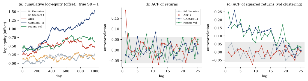
Each family is normalized so that the unconditional daily mean is \mu and the unconditional daily standard deviation is exactly \sigma; the target parameter \mathrm{SR}= \sqrt{252}\,\mu/\sigma is therefore known by construction, not estimated. With z_t \sim \mathcal N(0,1) iid: \begin{align} \textsf{iid Gaussian:}\quad & r_t = \mu + \sigma z_t,\\ \textsf{iid Student-}t\textsf{:}\quad & r_t = \mu + \sigma\, t_{\nu,t}\big/\sqrt{\nu/(\nu-2)}, \qquad \nu > 4,\\ \textsf{AR(1):}\quad & r_t = \mu + x_t,\quad x_t = \phi x_{t-1} + \varepsilon_t,\quad \mathrm{sd}(\varepsilon) = \sigma\sqrt{1-\phi^2}, \label{eq:ar1}\\ \textsf{GARCH(1,1):}\quad & r_t = \mu + s_t z_t,\quad s_t^2 = \omega + \alpha (s_{t-1}z_{t-1})^2 + \beta s_{t-1}^2,\quad \omega = \sigma^2(1-\alpha-\beta), \label{eq:garch}\\ \textsf{regime vol:}\quad & r_t = \mu + \sigma_{S_t} z_t,\quad S_t \in \{\text{low},\text{high}\} \text{ a 2-state Markov chain}. \label{eq:regime} \end{align} The AR(1) is started from its stationary law (x_0\sim\mathcal N(0,\sigma^2)), so it is exactly stationary with unconditional variance \sigma^2. The GARCH intercept \omega pins the unconditional variance at \sigma^2 analytically (initialized at \sigma^2 with a 500-step burn-in). The regime-switching state volatilities (\sigma_{\text{low}}, \sigma_{\text{high}}) solve \pi_{\text{low}}\sigma_{\text{low}}^2 + \pi_{\text{high}}\sigma_{\text{high}}^2 = \sigma^2 under the chain’s stationary distribution, given the ratio \sigma_{\text{high}}/\sigma_{\text{low}}, and S_0 is drawn from the stationary distribution. Serial dependence thus changes the sampling distribution of \widehat\mathrm{SR}—exactly what coverage measures—while the plug-in estimator remains consistent for the same known \mathrm{SR} under every family. Figure 1 shows one sample path per family and the dependence signatures the methods must cope with: only the AR(1) puts autocorrelation into returns; GARCH and regime volatility put it into squared returns.
Sampled design.
Every experiment draws its own fully recorded configuration: true annualized Sharpe uniform on [0,2]; daily volatility uniform on [0.005,0.02] (roughly 8–32\% annualized); the drift is then set to \mu = \mathrm{SR}\,\sigma/\sqrt{252} so the true Sharpe is exact by construction. Family-specific parameters: \nu\in\{5,6,8,12,20\}; \phi\in\{0.05,0.10,0.20,0.30\}; GARCH \alpha uniform on [0.03,0.12] with persistence \alpha+\beta uniform on [0.85,0.98]; regime volatility ratio uniform on [2,4] with stay probabilities uniform on [0.95,0.99] (low state) and [0.90,0.98] (high state). There are no hidden per-draw constants: every sampled parameter of every experiment is recorded in the released data, and the sampling ranges themselves are recorded in the results metadata.
Experimental setup
Sharpe coverage.
We run 400 experiments per (family, T) cell over T\in\{250,1000,4000\}—6{,}000 experiments in all. Each experiment generates one sample, builds all fourteen intervals at 90\% and 95\% nominal from that same sample (B=2{,}000), and records whether each interval covers the known true Sharpe, plus its width. Coverage estimates carry Wilson 95\% binomial intervals; with several hundred such intervals across the coverage tables, a handful of borderline significance calls are expected by multiplicity alone, so we lean on patterns across cells rather than single bold entries. At n=400 per cell the Wilson half-width is about \pm 0.02–0.04.
Maximum drawdown.
For each family we fix one canonical mid-range configuration (true \mathrm{SR}=1, \sigma=1\%/day; \nu=6; \phi=0.2; \alpha=0.08,\beta=0.88; volatility ratio 3 with stay probabilities 0.98/0.95) and T\in\{250,1000\}. The true sampling distribution of the length-T maximum drawdown is estimated once per configuration from 20{,}000 independent paths (seeded and cached). Each of 150 experiments per (family, T) cell—1{,}500 in all—then draws one sample, lets every eligible method predict the q-quantile \hat q of the drawdown distribution, and records the realized tail probability F_{\text{true}}(\hat q) = \mathbb P_{\text{true}}(\mathrm{MDD}\le \hat q). For a calibrated method the mean realized probability equals the nominal q.
Reproducibility.
Every experiment receives its own SeedSequence-spawned
generator in a fixed order, so all numbers are bit-identical regardless
of worker count. The full run takes about six minutes on a laptop (331 s in the released results).
Results
Where the advice holds: iid returns, heavy tails included
Table 1 pools the 2{,}400 experiments on the two iid families. The practitioner recipe is calibrated where its assumption holds: at 95\% nominal the iid percentile bootstrap covers 0.954 [0.945,0.961], the basic and BCa variants 0.952, and Lo’s iid standard error 0.953. The trade-level resamplers sit between 0.93 and 0.95: the 5-day and threshold-crossing (CUSUM) segmentations are calibrated (0.948 and 0.949), while the 21-day segmentation undercovers mildly (0.931)—not because of dependence (there is none) but because at T=250 it leaves only \lfloor 250/21\rfloor = 11 resampling units, too few for stable tail quantiles. The same small-T inefficiency, amplified, explains the fixed long-block stationary bootstraps: L=20 covers 0.932 and L=50 only 0.907 at 95\% pooled. The automatic-length block bootstraps are indistinguishable from the iid bootstrap here (0.953, 0.950)—on iid data the Politis–White rule correctly collapses to a mean block length of about 1.0–1.1 days, i.e. it recovers the iid bootstrap.
Heavy tails do not break the percentile bootstrap. On the Student-t family the percentile interval covers 0.945/0.938/0.970 at 95\% across T=250/1000/4000; restricting to the heaviest tail sampled (\nu=5, where the fourth moment barely exists, n=266) gives 0.962 at 95\% and 0.906 at 90\%. Lo’s normal-theory standard error survives these tails as well at the sample sizes studied. The failures documented below are therefore not about tails; they are about dependence.
| Method | coverage at 90\% nominal | coverage at 95\% nominal |
|---|---|---|
| Lo iid SE | 0.902 [0.890, 0.914] | 0.953 [0.944, 0.961] |
| Lo HAC SE | 0.897 [0.884, 0.908] | 0.949 [0.940, 0.957] |
| iid boot (percentile) | 0.902 [0.889, 0.913] | 0.954 [0.945, 0.961] |
| iid boot (basic) | 0.903 [0.891, 0.915] | 0.952 [0.943, 0.960] |
| iid boot (BCa) | 0.902 [0.890, 0.914] | 0.952 [0.942, 0.960] |
| trade resample (5d) | 0.892 [0.879, 0.904] | 0.948 [0.938, 0.956] |
| trade resample (21d) | 0.876 [0.862, 0.889] | 0.931 [0.920, 0.940] |
| trade resample (cusum) | 0.893 [0.880, 0.905] | 0.949 [0.939, 0.957] |
| stationary L{=}5 | 0.895 [0.882, 0.906] | 0.951 [0.941, 0.959] |
| stationary L{=}10 | 0.885 [0.872, 0.897] | 0.943 [0.932, 0.951] |
| stationary L{=}20 | 0.874 [0.860, 0.886] | 0.932 [0.922, 0.942] |
| stationary L{=}50 | 0.845 [0.830, 0.859] | 0.907 [0.895, 0.918] |
| stationary auto | 0.901 [0.888, 0.912] | 0.953 [0.943, 0.960] |
| circular auto | 0.900 [0.887, 0.911] | 0.950 [0.940, 0.958] |
Autocorrelation breaks iid resampling—asymptotically
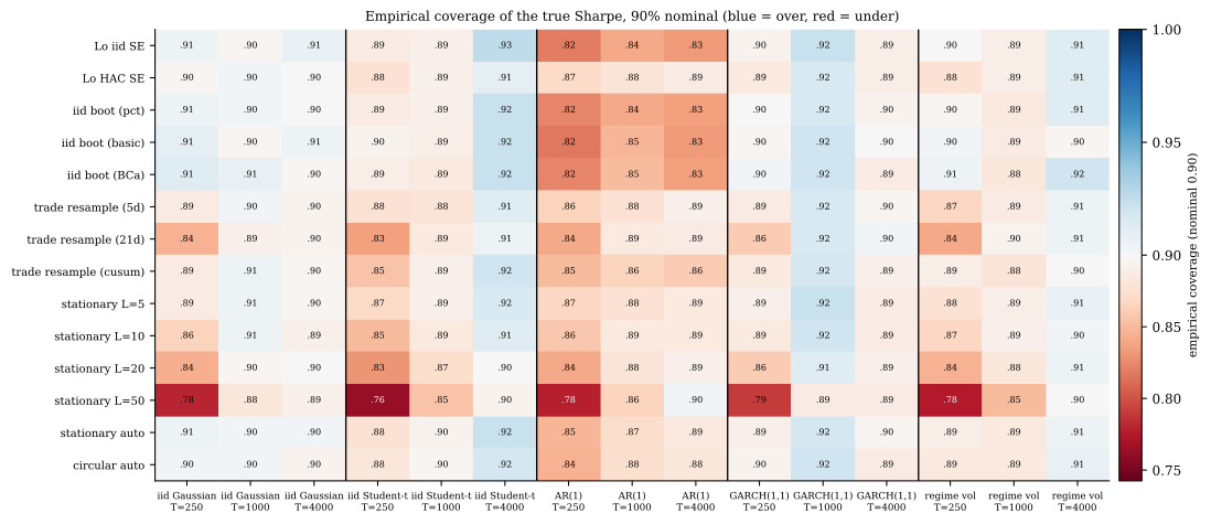
Table 2 is the headline: coverage at 95\% nominal on the three dependent families,
stratified by T (the 90\% panorama over all fifteen family\times T cells is Figure 2; the full table with Wilson intervals
and widths is in the released results.json). Two of the
three dependent families turn out to be nearly harmless for Sharpe
coverage. Under GARCH(1,1) and regime-switching volatility the iid
percentile bootstrap covers 0.885–0.915 at 90\% nominal across all cells, and binning
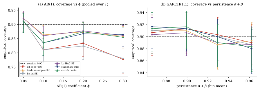
the GARCH experiments by persistence shows only a mild slide, from 0.907 in the lowest-persistence quartile to
0.890 in the highest (mean \alpha+\beta = 0.962; Figure 3b). The reason is structural:
these processes leave the level of returns serially
uncorrelated, and the sampling variance of the Sharpe estimator is
driven by the long-run covariance of (r_t,
r_t^2)—volatility clustering enters only through the second
component, a second-order effect at these persistence levels, sample
sizes, and Sharpe levels (daily \mathrm{SR} is at most 0.13 in our designs, which suppresses the
r_t^2 channel’s weight).
| AR(1) | GARCH(1,1) | regime vol | |||||||
| Method | 250 | 1000 | 4000 | 250 | 1000 | 4000 | 250 | 1000 | 4000 |
| Lo iid SE | 0.892 | 0.892 | 0.910 | 0.953 | 0.963 | 0.958 | 0.948 | 0.938 | 0.953 |
| Lo HAC SE | 0.938 | 0.927 | 0.958 | 0.948 | 0.968 | 0.960 | 0.948 | 0.945 | 0.953 |
| iid boot (percentile) | 0.885 | 0.892 | 0.907 | 0.950 | 0.960 | 0.955 | 0.950 | 0.938 | 0.953 |
| iid boot (basic) | 0.900 | 0.900 | 0.900 | 0.960 | 0.968 | 0.950 | 0.948 | 0.938 | 0.948 |
| iid boot (BCa) | 0.887 | 0.890 | 0.907 | 0.953 | 0.968 | 0.958 | 0.948 | 0.940 | 0.950 |
| trade resample (5d) | 0.943 | 0.925 | 0.955 | 0.943 | 0.963 | 0.960 | 0.935 | 0.935 | 0.948 |
| trade resample (21d) | 0.895 | 0.935 | 0.953 | 0.915 | 0.960 | 0.953 | 0.895 | 0.938 | 0.943 |
| trade resample (cusum) | 0.895 | 0.907 | 0.925 | 0.943 | 0.965 | 0.955 | 0.943 | 0.938 | 0.950 |
| stationary L{=}5 | 0.935 | 0.925 | 0.950 | 0.940 | 0.968 | 0.963 | 0.938 | 0.935 | 0.953 |
| stationary L{=}10 | 0.930 | 0.930 | 0.953 | 0.932 | 0.963 | 0.958 | 0.925 | 0.935 | 0.948 |
| stationary L{=}20 | 0.907 | 0.922 | 0.955 | 0.912 | 0.953 | 0.953 | 0.897 | 0.935 | 0.940 |
| stationary L{=}50 | 0.845 | 0.910 | 0.955 | 0.863 | 0.940 | 0.943 | 0.868 | 0.912 | 0.940 |
| stationary auto | 0.917 | 0.922 | 0.953 | 0.950 | 0.963 | 0.960 | 0.945 | 0.935 | 0.953 |
| circular auto | 0.912 | 0.927 | 0.948 | 0.955 | 0.968 | 0.953 | 0.945 | 0.932 | 0.948 |
Autocorrelation is a different story. Figure 3a tracks 90\%-nominal coverage against the AR(1) coefficient (pooled over T, roughly 300 experiments per \phi value): the iid percentile bootstrap degrades from 0.915 at \phi=0.05 to 0.811, 0.834, and 0.777 at \phi=0.10, 0.20, 0.30 (adjacent-\phi differences are within Wilson noise; it is the trend, not each step, that is monotone). Table 3 zooms into the worst cell, \phi=0.3 (n=296). At 95\% nominal the per-bar iid bootstrap covers 0.841 [0.795,0.878]: an interval sold as missing 5\% of the time misses 15.9\% of the time, more than three times the nominal rate.
Two features make this failure structural rather than incidental. First, it does not vanish with sample size: at 95\% nominal the per-T coverage at \phi=0.3 is 0.812, 0.856, 0.854 for T=250,1000,4000 (at 90\%: 0.719, 0.798, 0.812). The iid bootstrap converges—to an interval calibrated for the wrong sampling variance. Under positive autocorrelation the variance of \widehat\mathrm{SR} is inflated by a factor that survives T\to\infty, and intervals built from independently resampled bars are too narrow by exactly that factor, at every sample size: the limiting coverage of an iid-variance interval under AR(1) is 2\Phi\!\big(z_{\alpha/2}\sqrt{(1-\phi)/(1+\phi)}\big)-1, which at \phi=0.3 equals 0.850 at 95\% nominal and 0.773 at 90\%—our T=4000 cells (0.854 and 0.812) sit on that asymptote. (Per-T cells have n\approx 96–104, Wilson half-width {\sim}0.07, so the supported per-T statement is that T=4000 coverage still significantly excludes nominal, not that adjacent T cells differ.) Second, the interval construction is irrelevant: percentile 0.841, basic 0.848, BCa 0.838. The BCa machinery corrects bias and skewness of the bootstrap distribution; it cannot correct a bootstrap distribution whose dispersion is wrong. Lo’s iid standard error fails identically (0.841)—it shares the assumption, not the mechanism. What fixes the cell is modeling the dependence: Lo’s HAC variant covers 0.946, the 5-day trade resampler 0.946, the circular block bootstrap 0.946, the automatic stationary bootstrap 0.939.
| pooled over T | 95\% nominal, by T | ||||
| Method | at 90\% | at 95\% | 250 | 1000 | 4000 |
| Lo iid SE | 0.780 | 0.841 | 0.812 | 0.856 | 0.854 |
| Lo HAC SE | 0.861 | 0.946 | 0.917 | 0.952 | 0.969 |
| iid boot (percentile) | 0.777 | 0.841 | 0.812 | 0.856 | 0.854 |
| iid boot (basic) | 0.780 | 0.848 | 0.823 | 0.865 | 0.854 |
| iid boot (BCa) | 0.780 | 0.838 | 0.812 | 0.846 | 0.854 |
| trade resample (5d) | 0.858 | 0.946 | 0.927 | 0.952 | 0.958 |
| trade resample (21d) | 0.858 | 0.929 | 0.865 | 0.962 | 0.958 |
| trade resample (cusum) | 0.828 | 0.875 | 0.844 | 0.894 | 0.885 |
| stationary L{=}5 | 0.855 | 0.932 | 0.885 | 0.952 | 0.958 |
| stationary L{=}10 | 0.868 | 0.929 | 0.865 | 0.952 | 0.969 |
| stationary L{=}20 | 0.872 | 0.929 | 0.865 | 0.962 | 0.958 |
| stationary L{=}50 | 0.851 | 0.905 | 0.812 | 0.942 | 0.958 |
| stationary auto | 0.865 | 0.939 | 0.885 | 0.962 | 0.969 |
| circular auto | 0.855 | 0.946 | 0.906 | 0.962 | 0.969 |
The trade-resampling nuance: an accidental block bootstrap
The practitioner recipe’s preferred unit is the trade, not the bar, and this turns out to matter enormously—in the recipe’s favor. Resampling fixed-length 5-day episodes is algebraically a non-overlapping block bootstrap with block length 5, and five days comfortably exceeds the dependence length of an AR(1) with \phi\le0.3 (autocorrelation 0.3^5\approx0.002 five bars out). Accordingly, at \phi=0.3 and 95\% nominal the 5-day trade resampler covers 0.946 [0.914,0.966] where the per-bar iid bootstrap covers 0.841 [0.795,0.878] (Table 3)—fully calibrated, by accident of unit choice rather than by design.
The conditions for the accident to work are visible in the same tables. The unit must exceed the dependence length: the threshold-crossing (CUSUM) segmentation produces episodes averaging about 6 days on the AR(1) family (5.6 at \phi=0.3), but their lengths are variable and data-dependent—fast threshold crossings produce many short episodes—and its coverage lands in between, 0.875 at \phi=0.3 (95\%), significantly under nominal. And the number of units must stay large: the 21-day segmentation handles the dependence (0.962 at \phi=0.3, T=1000) but undercovers at T=250 (0.865) for the same reason it undercovers on iid data there—eleven resampling units cannot pin a 95\% quantile. The per-bar version of the recipe is simply the degenerate case: a “trade” of one bar, which is the failure mode of Section 6.2.
This reframes the practitioner advice rather than vindicating or damning it: “resample trades” is sound when trades are multi-day episodes, because it is then an unwitting block bootstrap whose block structure happens to match the dependence; it is unsound when the resampling unit is a bar, a one-day trade, or an episode distribution with many short members.
Block length: the sweep, the automatic rule, and what width buys
The fixed-length sweep quantifies the block-length dilemma. Long blocks pay a small-sample price: at T=250 and 90\% nominal, L=50 covers 0.781 pooled over the dependent families (0.762–0.790 per family, including the iid ones)—with only five distinct blocks per resample, the bootstrap distribution is too coarse and too narrow. Yet long blocks are exactly what large-T dependence wants: at T=4000 on AR(1), L=50 is the best method in the column (0.902 at 90\%). No fixed L wins everywhere.
The automatic Politis–White rule navigates this trade-off about as well as a data-driven rule can, and is one of the two methods we would recommend as a default, but it is not magic. On iid families it correctly collapses to L\approx 1 and reproduces the iid bootstrap. On AR(1) it chooses mean lengths that grow with T and \phi (\approx 3.8/6.1/10.9 days at \phi=0.3 for T=250/1000/4000) yet still undercovers, by 3.2 points at 90\% nominal pooled over the AR(1) family (0.868) and 1.9 points at 95\% (0.931). Part of this is the generic small-T difficulty (below), and part is that the rule optimizes the block length for the long-run variance of the sample mean, not for quantiles of a studentized ratio statistic [6, 21]; its chosen lengths are, for this purpose, slightly short.
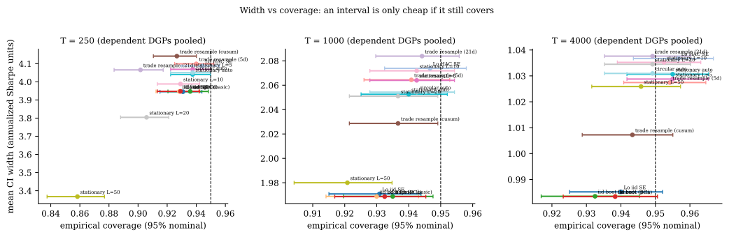
Two cross-method facts deserve emphasis. First, at T=250 on the dependent families, no method reaches nominal 90\% coverage: the best of the fourteen achieves 0.879, and every Wilson interval excludes 0.90. At 95\% nominal only Lo’s HAC standard error (0.944) and the 5-day trade resampler (0.940) are not significantly under. One year of daily data is simply not enough for honest dependence-aware interval estimation at conventional levels, by any of these methods. Second, the width–coverage trade-off (Figure 4) shows there is no free narrowness: at T=250 the methods that approach nominal coverage do so with intervals about 4.1 annualized-Sharpe units wide (\pm 2 around the estimate)—an honest statement of how little one year of daily data constrains a Sharpe ratio—while the narrow intervals (L=50 at width 3.4) buy their width by not covering. Pooling can also flatter a method: at T=4000 the BCa interval is not significantly under nominal pooled across the dependent families (0.938), yet its AR(1) stratum sits at 0.907 (Table 2)—averaging the harmless GARCH and regime columns into the harmful AR(1) one hides the failure that matters. Coverage claims should be read stratified.
Maximum drawdown: optimistic everywhere
The drawdown study asks each bootstrap to predict the 5\% worst-case quantile of the maximum-drawdown distribution—the number a practitioner quotes as “with 95\% probability the drawdown will not be deeper than this”—and scores the realized exceedance probability against the 20{,}000-path truth. Table 4 reports the result: every method is optimistic on every DGP. Even on iid Gaussian returns, where the resampling scheme is correct, the realized exceedance of the iid bootstrap’s q_{0.05} prediction is 0.102 at T=250 and 0.082 at T=1000—roughly double nominal. The bootstrap sees only one realized path; its resamples cannot produce drawdowns much deeper than the volatility and luck of that one path allow, so the predicted tail quantile inherits estimation noise asymmetrically. This is a plug-in bias, not a dependence effect, and it decays only slowly with T.
Dependence then stacks on top. Under AR(1) the per-bar iid bootstrap’s exceedance is 0.232 at T=250 and 0.226 at T=1000—the “5\%” drawdown is a one-in-four event, and the bias does not shrink with the path length, for the same structural reason as in Section 6.2. Block methods repair most of this channel: at T=1000 the automatic stationary bootstrap brings the AR(1) exceedance from 0.226 down to 0.115, the 5-day trade resampler to 0.112 (at T=250 they reach only 0.196 and 0.143). But under regime-switching volatility—returns uncorrelated, variance persistent—block resampling fixes essentially nothing: 0.165\to0.168 at T=250, 0.134\to0.133 at T=1000. The blocks are far shorter than the regimes, so no resampling scheme in our set reproduces the possibility that the next path spends most of its life in the high-volatility state. GARCH sits in between (0.115/0.106 iid bootstrap, unimproved by blocks). Note the contrast with Section 6.2: volatility dynamics that barely move Sharpe coverage substantially poison drawdown tails—the drawdown is an extreme path functional and feels the clustering that the Sharpe estimator’s CLT averages out.
Even the predicted median drawdown is biased under autocorrelation: the per-bar bootstrap’s q_{0.50} is exceeded with probability 0.661 (T=250) and 0.696 (T=1000) on AR(1), versus 0.51–0.61 for the block methods. In relative terms the per-bar q_{0.05} prediction is about 15–17\% too shallow on AR(1). Across our grid the realized probability of the nominal 5\% drawdown ranges from 0.07 to 0.23: a practitioner quoting a bootstrap “5\% worst-case drawdown” should expect the true exceedance probability to be 1.5–5 times larger.
| Family | T | iid pct | trade-5d | SB L{=}20 | SB auto | CB auto |
|---|---|---|---|---|---|---|
| iid Gaussian | 250 | 0.102 | 0.111 | 0.161 | 0.102 | 0.102 |
| 1000 | 0.082 | 0.088 | 0.108 | 0.082 | 0.083 | |
| iid Student-t | 250 | 0.093 | 0.118 | 0.163 | 0.093 | 0.094 |
| 1000 | 0.074 | 0.077 | 0.094 | 0.074 | 0.074 | |
| AR(1) | 250 | 0.232 | 0.143 | 0.182 | 0.196 | 0.193 |
| 1000 | 0.226 | 0.112 | 0.121 | 0.115 | 0.111 | |
| GARCH(1,1) | 250 | 0.115 | 0.138 | 0.176 | 0.118 | 0.115 |
| 1000 | 0.106 | 0.110 | 0.138 | 0.105 | 0.105 | |
| regime vol | 250 | 0.165 | 0.181 | 0.227 | 0.168 | 0.169 |
| 1000 | 0.134 | 0.133 | 0.162 | 0.133 | 0.133 |
Discussion
The practitioner advice should be split into verdicts by regime and by statistic, and each verdict is quantitative.
For the Sharpe ratio on genuinely iid PnL, the advice is simply correct: every variant—per-bar percentile bootstrap, trade resampling, Lo’s closed form—is calibrated, heavy tails included (Table 1). Nothing in our results justifies abandoning the iid bootstrap where independence is credible.
For the Sharpe ratio under autocorrelated PnL—overlapping positions, slow signals, smoothed marks—per-bar iid resampling should never be used. Its failure is not a finite-sample blemish that more data cures: at \phi=0.3 the 95\% interval misses 15–19\% of the time at every sample length up to T=4000, and upgrading the interval construction to BCa changes nothing because the resampling scheme, not the quantile formula, is wrong. The fix costs one line of code: a stationary or circular block bootstrap with the corrected Politis–White automatic length, or Lo’s HAC standard error. Both are nearly calibrated everywhere here, with two honest caveats: expect roughly 2–3 points of residual undercoverage on autocorrelated data at T\le1000, and expect no method to deliver nominal 90\% coverage at T=250 on dependent data—at that length the honest interval is about \pm2 annualized Sharpe units wide, which is itself the finding.
For trade-level resampling, the verdict depends on the unit. Resampling whole multi-day trades is an accidental non-overlapping block bootstrap and inherits its calibration when the typical trade is longer than the dependence length and the trade count is large (0.946 at \phi=0.3 for 5-day episodes); it degrades when episode lengths are variable with many short members (CUSUM, 0.875) and collapses to the per-bar failure as trades approach one bar. A practitioner who wants to keep the trade-resampling workflow should check the trade-length distribution against the PnL autocorrelation length, and prefer the automatic block bootstrap when in doubt—it needs no such check.
For maximum drawdown, bootstrap quantiles should be treated as optimistic lower bounds on the severity of the tail, under every method tested. Block schemes remove the autocorrelation-driven part of the bias but none of the volatility-regime part, and even the iid-on-iid case runs at twice the nominal exceedance. A reported “5\% worst-case drawdown” from 250–1000 days of data behaved, in our grid, like a 7–23\% event; multiplying the nominal tail probability by a factor of 1.5 to 5, or validating the quantile against a parametric vol-clustering model, is the prudent reading.
Limitations
Our DGPs are stylized in disclosed ways. Innovations are Gaussian in the dependent families, so heavy tails and dependence are never combined (the Student-t family is iid); AR(1) dependence is capped at \phi=0.3, and real overlapping-position PnL can be more persistent; the regime and GARCH parameter ranges, while drawn to be realistic, are choices. The trade-level method is scored under a charitable reading—we resample trade episodes but recompute the daily-frequency Sharpe, isolating the resampling question from the per-trade units error in the circulated recipe; the fixed segmentation drops a sub-window remainder, and the CUSUM threshold uses the full-sample standard deviation, as a practitioner would compute it. We evaluate percentile intervals for the block bootstraps as practitioners use them; studentized block intervals with higher-order refinements [12] could narrow the residual small-T gap and are not tested. The Politis–White rule is applied as published (it optimizes the sample-mean long-run variance, not ratio-statistic quantiles). The drawdown truth is itself a 20{,}000-path Monte Carlo estimate (its quantile error is negligible relative to the reported effects, though it is shared within a cell and so does not average out across experiments), computed at one canonical parameter point per family and T\in\{250,1000\} only. Finally, true Sharpe ratios are sampled from [0,2] and all streams are univariate daily PnL: selection across many backtests [2, 22], transaction costs, and multi-asset effects are out of scope.
Conclusion
We gave the “bootstrap your backtest” advice its first controlled coverage test, across fourteen interval methods, five data-generating processes with exactly known annualized Sharpe ratios, and three sample lengths. The verdict splits cleanly. On iid returns the advice is calibrated, heavy tails included: the pooled 95\% percentile-bootstrap coverage is 0.954. Under autocorrelation the per-bar version is broken asymptotically, not just in small samples—0.841 coverage at 95\% nominal for \phi=0.3, unimproved from T=250 to T=4000 and unrescued by BCa—because the iid resampling scheme converges to the wrong sampling variance. Resampling multi-day trades is an accidental non-overlapping block bootstrap and is calibrated whenever the trade unit exceeds the dependence length and trades are plentiful, which is the regime in which the practitioner recipe quietly works. Automatic-length block bootstraps and Lo’s HAC standard error are the best general-purpose defaults, within 2–3 points of nominal everywhere except T=250, where no method reaches nominal on dependent data. And for maximum drawdown every bootstrap tested is optimistic on every process: the nominal 5\% worst-case drawdown realized with probability 0.07–0.23, with block methods fixing only the autocorrelation channel. Resample blocks, not bars; report stratified coverage, not pooled comfort; and read bootstrap drawdown quantiles as lower bounds.
Reproducibility.
All experiments are deterministic given the released seeds, and the
worker count changes wall time only, never numbers. A single command
(python scripts/run_all.py) regenerates every number in
about six minutes on a laptop, the package’s figures module
regenerates every figure, and the script
check_paper_numbers.py asserts that every value quoted in
this paper’s tables and text matches the generated results. The DGPs,
interval constructors, drawdown truth cache, and analysis are released
as an open-source package with tests.
References
The specific trade-level resampling recipe we test, including the choice of the trade as the resampling unit, follows the author’s own earlier practitioner writing (a market-making blog post on Monte Carlo analysis of backtests). This paper is a controlled self-audit of advice the author has himself circulated, not an attack on a third party.↩︎
The recipe as circulated literally computes \mathrm{mean}/\mathrm{std}\times\sqrt{252} on per-trade returns, which targets a different parameter whenever trades span more than one day; scoring that version would conflate a units error with the resampling question, so we score this charitable reading throughout.↩︎